Chance is a Fine Thing
It used to be said that you go to Las Vegas to get married and to Reno to get a divorce. Now you can visit both cities for their slot machines. With 100 slot machines, Reno’s Peppermill Casino isn’t even the largest casino in town. Walking through its main hall, the roulette and blackjack tables were shadowy and subdued in comparison to the flashing, spinning, beeping regiments of slots. Technological evolution has deprived most one-armed bandits of their lever limbs and mechanical insides. Players now bet by pressing lit buttons or touch-screen displays. Occasionally I heard the rousing sound of clattering change, but this came from pre-recorded samples since coins have been replaced by electronic credits.
Slots are the casino industry’s cutting edge; its front line and its bottom line. The machines make $25 billion a year in the United States (after they’ve paid out all their prize money), which is about two and a half times the total value of movie tickets sold in the country annually. In Nevada, the global centre of casino culture, slots now make up almost 70 percent of gambling revenue – and the number nudges higher every year.
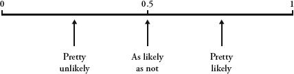
Probability is the study of chance. When we flip a coin, or play the slots, we do not know how the coin will land, or where the spinning reels will stop. Probability gives us a language to describe how likely it is that the coin will come up heads, or that we will hit the jackpot. With a mathematical approach, unpredictability becomes very predictable. While we take this idea for granted in our daily lives – it is implicit, for example, whenever we read the weather forecast – the realization that maths can tell us about the future was a very profound and comparatively recent idea in the history of human thought.
I had come to Reno to meet the mathematician who sets the odds for more than half of the world’s slot machines. His job has historical pedigree – probability theory was first conceived in the sixteenth century by the gambler Girolamo Cardano, our Italian friend we met earlier when discussing cubic equations. Rarely, however, has a mathematical breakthrough arisen from such self-loathing. ‘So surely as I was inordinately addicted to the chess board and the dicing table, I know that I must rather be considered deserving of the severest censure,’ he wrote. His habit yielded a short treatise called The Book on Games of Chance, the first scientific analysis of probability. It was so ahead of its time, however, that it was not published until a century after his death.
Cardano’s insight was that if a random event
has several equally likely outcomes, the chance of any individual
outcome occurring is equal to the proportion of that outcome to all
possible outcomes. This means that if there is a one-in-six chance
of something happening, then the chance of it happening is one
sixth. So, when you roll a die, the chance of getting a six is
 . The
chance of throwing an even number is
. The
chance of throwing an even number is  . The chance of throwing an
even number is . which is the same as
. The chance of throwing an
even number is . which is the same as  . Probability can be defined
as the likelihood of something happening expressed as a fraction.
Impossibility has a probability of 0; certainty, a probability of
1; and the rest is in between.
. Probability can be defined
as the likelihood of something happening expressed as a fraction.
Impossibility has a probability of 0; certainty, a probability of
1; and the rest is in between.
This seems straightforward, but it isn’t. The Greeks, the Romans and the ancient Indians were all obsessive gamblers. None of them, though, attempted to understand how randomness is governed by mathematical laws. In Rome, for exale, coins were flipped as a way of settling disputes. If the side with the head of Julius Caesar came up, it meant that he agreed with the decision. Randomness was not seen as random, but as an expression of divine will. Throughout history, humans have been remarkably imaginative in finding ways to interpret random events. Rhapsodomancy, for example, was the practice of seeking guidance through chance selection of a passage in a literary work. Similarly, according to the Bible, picking the short straw was an impartial way of selecting only in so far as God let it be that way: ‘The lot is cast into the lap; but the whole disposing thereof is of the Lord’ (Proverbs 16: 33).
Superstition presented a powerful block against a scientific approach to probability, but after millennia of dice-throwing, mysticism was overcome by perhaps a stronger human urge – the desire for financial profit. Girolamo Cardano was the first man to take Fortune hostage. It could be argued, in fact, that the invention of probability was the root cause of the decline, over the last few centuries, of superstition and religion. If unpredictable events obey mathematical laws, there is no need to have them explained by deities. The secularization of the world is usually associated with thinkers such as Charles Darwin and Friedrich Nietzsche, yet quite possibly the man who set the ball rolling was Girolamo Cardano.
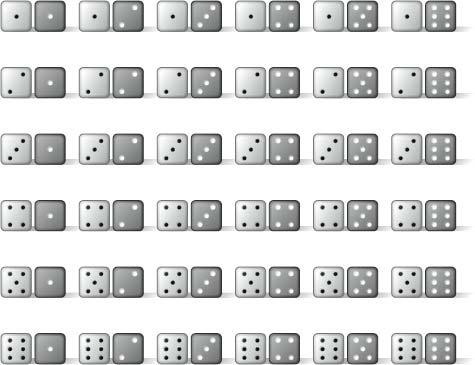
Games of chance have most commonly involved dice. A model popular in antiquity was the astragalus – an anklebone from a sheep or a goat – that had four distinctly flat faces. Indians liked dice in the shape of rods and Toblerones, and they marked the different faces with pips, the most likely explanation for which is that dice predate any formal system of numerical notation, and this tradition has survived. The fairest dice have identical sides, and if one imposes the further condition that each side must also be a regular polygon, there are only five shapes that fit the bill, the Platonic solids. All the Platonic solids have been used as dice. Ur, possibly the world’s oldest known game, which dates from at least as far back as the third century bc, used a tetrahedron, which, however, is the worst of the five choices because the tetrahedron hardly rolls and has only four sides. Octahedrons (eight sides) were used in ancient Egypt, and dodecahedrons (twelve) and icosahedrons (twenty) are still found in fortune-tellers’ handbags.
By far the most popular dice shape has been the cube. It is the easiest to make, its span of digits is neither too big nor too small, it rolls nicely but not too easily, and it’s obvious on which number it lands. Cubical dice with pips are a cross-cultural symbol of luck and chance, as comfortable bashed around in Chinese mah-jong salons as they are dangling from the rear-view mirrors of British cars.
As I mentioned earlier, roll one die and the
chance of a six is . Roll another die and the chance of a six is also
. What is
the chance of rolling a pair of dice and getting a pair of sixes?
The most basic rule of probability is that the chances of two
independent events happening is the same thing as the chance of one
event happening multiplied
by the chance of the second event happening. When you throw a pair
of dice the outcome of the first die is independent of the outcome
of the second, and vice versa. So, the chances of throwing two
sixes is
× , or
 . You can
see this visuallgits iounting all the possible combinations of two
dice: there are 36 equally likely outcomes and only one of them is
a six and a six.
. You can
see this visuallgits iounting all the possible combinations of two
dice: there are 36 equally likely outcomes and only one of them is
a six and a six.
Conversely, of the 36 possible outcomes, 35 of
them are not double six.
So, the probability of not throwing a six and a six is  . Rather than
counting up 35 examples, you can equally start with the full set
and then subtract the instances of double sixes. In this example, 1
–
=. The
probability of something not happening, therefore, is 1 minus the
probability of that thing happening.
. Rather than
counting up 35 examples, you can equally start with the full set
and then subtract the instances of double sixes. In this example, 1
–
=. The
probability of something not happening, therefore, is 1 minus the
probability of that thing happening.
The dicing table was an early equivalent of the slot machine, where gamblers placed wagers on the outcome of dice throws. One classic gamble was to roll four dice and bet on the chance of at least one six appearing. This was a nice little earner for anyone willing to put money on it, and we already have enough maths knowledge to see why:
Step 1: The probability of rolling a six in four rolls of dice is the same as 1 minus the probability of not getting a six on any of the four dice.
Step 2: The probability of not getting a six on one die is
, so if there are four dice, the probability is
which is 0.482.
Step 3: So, the probability of rolling a six is 1 – 0.482 = 0.518.
A probability of 0.518 means that if you threw four dice a thousand times, you could expect to get at least one six about 518 times, and get no sixes about 482 times. If you gambled on the chance of at least one six, you would win on average more than you would lose, so you would end up profiting.
The seventeenth-century writer Chevalier de Méré was a regular at the dicing table, as he was at the most fashionable salons in Paris. The chevalier was as interested in the mathematics of dicing as he was in winning money. He had a couple of questions about gambling, though, that he was unable to answer himself, so in 1654 he approached the distinguished mathematician Blaise Pascal. His chance enquiry was the random event that set in motion the proper study of randomness.
Blaise Pascal was only 31 when he received de Méré’s queries, but he had been known in intellectual circles for almost two decades. Pascal had shown such gifts as a young child that at 13 his father had let him attend the scientific salon organized by Marin Mersenne, the friar and prime-number enthusiast, which brought together many famous mathematicians, including René Descartes and Pierre de Fermat. While still a teenager, Pascal proved important theorems in geometry and invented an early mechanical calculation machine, which was called the Pascaline.
The first question de Méré asked of Pascal
concerned double sixes. As we saw above, there is a chance of getting
double six when you throw two dice. The overall chance of getting a
double six increases the more times you throw the pair of dice. The
chevalier wanted to know how many times he needed to throw the dice
to make gambling on the occurrence of a double six a good bet.
His second question was more complex. Say Jean and Jacques are playing a dice game consisting of several rounds in which both roll a die to see who gets the highest number. The outright winner is whoever rolls the highest number three times. Each has a stake of 32 francs, so the pot is 64 francs. If the game has to be terminated after three rounds, when Jean has rolled the highest number twice and Jacques once, how should the pot be divided up?
Pondering the answers, and feeling the need to discuss them with a fellow genius, Pascal wrote to his old friend from the Mersenne salon, Pierre de Fermat. Fermat lived far from Paris, in Toulouse, an appropriately named city for someone analysing a problem about gambling. He was 22 years older than Pascal and worked as a judge at the local criminal court, dabbling in maths only as an intellectual recreation. Nevertheless, his amateur ruminations had made him one of the most respected mathematicians of the first half of the seventeenth century.
The short correspondence between Pascal and Fermat about chance – which they called hasard – was a landmark in the history of science. Between them the men solved both of the literary bon vivant’s problems, and in so doing, set the foundations of modern probability theory.
Now for the answers to Chevalier de Méré’s
questions. How many times do you need to throw a pair of dice so
that it is more likely than not that a double six will appear? In
one throw of two dice the chance of a double six is , or 0.028. The
chance of a double six appearing in two throws of two dice is 1
minus the probability of no double sixes appearing in two throws,
or 1 – (  ). This works out to be
  , or 0.055. (Note: the chance
of a double six in two throws is not
, or 0.055. (Note: the chance
of a double six in two throws is not  . This is the chance of a double six in both
throws. The probability we are concerned with is the chance of
at least one double six,
which includes the outcomes of either a double six in the first
throw, in the second throw, or in both throws. The gambler needs
only one double six to win, not a double six in both.) The chances
of a double six in three throws of two dice are 1 minus the
probability of no doubles, which this time is
. This is the chance of a double six in both
throws. The probability we are concerned with is the chance of
at least one double six,
which includes the outcomes of either a double six in the first
throw, in the second throw, or in both throws. The gambler needs
only one double six to win, not a double six in both.) The chances
of a double six in three throws of two dice are 1 minus the
probability of no doubles, which this time is 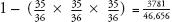 0.081. As we can see, the
more times one throws the dice, the higher the probability of
throwing a double six: 0.028 with one throw, 0.055 with two, and
0.081 with three. Therefore, the original question can be rephrased
as ‘After how many throws does this fraction exceed 0.5?’, as a
probability of more than a half means that the event is more likely
than not. Pascal calculated correctly that the answer is 25 throws.
If the chevalier gambled on the chance of a double six in 24
throws, he could expect to lose money, but after 25 throws, the
odds shift in his favour and he could expect to win.
0.081. As we can see, the
more times one throws the dice, the higher the probability of
throwing a double six: 0.028 with one throw, 0.055 with two, and
0.081 with three. Therefore, the original question can be rephrased
as ‘After how many throws does this fraction exceed 0.5?’, as a
probability of more than a half means that the event is more likely
than not. Pascal calculated correctly that the answer is 25 throws.
If the chevalier gambled on the chance of a double six in 24
throws, he could expect to lose money, but after 25 throws, the
odds shift in his favour and he could expect to win.
De Méré’s second question, about divvying up the pot, is often called the problem of points and had been posed before Fermat and Pascal tackled it, but never correctly resolved. Let’s restate the question in terms of heads and tails. Jean wins each round if the coin lands on heads, and Jacques wins if it lands on tails. The first person to win three rounds takes the pot of 64. With the score at two heads for Jean and one tails for Jacques, the game needs to come to an abrupttop. If this is the case, what’s the fairest way to divide the pot? One answer is that Jean should take the lot, since he is ahead, but this doesn’t take account of the fact that Jacques still has a chance of winning. Another answer is that Jean should take twice as much as Jacques, but again this is not fair because the 2–1 score reflects past events. It’s not an indication of what might happen in the future. Jean is not better at guessing coins than Jacques. Each time they throw, there is a 50:50 chance of the coin landing heads or tails. The best, and fairest, analysis is to consider what might happen in the future. If the coin is tossed another two times, the possible outcomes are:
heads, heads
heads, tails
tails, heads
tails, tails
After these two throws, the game has been won.
In the first three instances Jean wins, and in the fourth Jacques
does. The fairest way to divide the pot is for  to go to Jean and
 to go to
Jacques, so the cash is divided 48 francs to 16. This seems fairly
straightforward now, but in the seventeenth century the idea that
random events that haven’t yet taken place can be treated
mathematically was a momentous conceptual breakthrough. The concept
underpins our scientific understanding of much of the modern world,
from physics to finance and from medicine to market research.
to go to
Jacques, so the cash is divided 48 francs to 16. This seems fairly
straightforward now, but in the seventeenth century the idea that
random events that haven’t yet taken place can be treated
mathematically was a momentous conceptual breakthrough. The concept
underpins our scientific understanding of much of the modern world,
from physics to finance and from medicine to market research.
A few months after he first wrote to Fermat about the gambler’s queries, Pascal had a religious experience so intense that he scribbled a report of his trance on a piece of paper that he carried with him in a special pouch sewn into the lining of his jacket for the rest of his life. Perhaps the cause was the near-death accident in which his coach hung perilously off a bridge after the horses plunged over the parapet, or perhaps it was a moral reaction to the decadence of the dicing tables of pre-revolutionary France – in any case, it revitalized his commitment to Jansenism, a strict Catholic cult, and he abandoned maths for theology and philosophy.
Nonetheless, Pascal could not help but think mathematically. His most famous contribution to philosophy – an argument about whether or not one should believe in God – was a continuation of the new approach to analysing chance that he had first discussed with Fermat.
In simple terms, expected value is what you can expect to get out of a bet. For example, what could Chevalier de Méré expect to win by betting £10 on getting a six when rolling four dice? Imagine that he wins £10 if there is a six and loses everything if there is no six. We know that the chance of winning this bet is 0.518. So, just over half the time he wins £10, and just under half he loses £10. The expected value is calculated by multiplying the probability of each outcome with the value of each outcome, and then adding them up. In this case he can expect to win:
(chances of winning £10)×£10 + (chances of losing £10)×–£10
or
(0.518×£10) + (0.482×–£10) = £5.18 – £4.82 = 36p
(In this equation, money won is a positive number, and money lost is a negative number.) Of course, in no single bet will de Méré win 36p – either he wins £10 or he loses £10. The value of 36p is theoretical, but, on average, if he keeps on betting, his winnings will approximate 36p per bet.
Pascal was one of the first thinkers to exploit the idea of expected value. His mind, though, was occupied by much higher thoughts than the financial benefits of the dicing table. He wanted to know whether it was worth placing a wager on the existence of God.
Imagine, Pascal wrote, gambling on God’s existence. According to Pascal, the expected value of such a wager can be calculated by the following equation:
(chance of God existing)×(what you win if He exists) + (chance of God not existing)×(what you win if He doesn’t exist)
So, say the chances of God existing are 50:50;
that is, the probability of God’s existence is . If you believe in God,
what can you expect to get out of this bet? The formula
becomes:
(
In other words, betting on God’s existence is a very good bet because the reward is so fantastic. The arithmetic works out because half of nothing is nothing, but half of something infinite is also infinite. Likewise, if the chance of God existing is only a hundredth, the formula is:
(
×eternal happiness) + (
×nothing) = eternal happiness
Again, the rewards of believing that God exists are equally phenomenal, since one hundredth of something infinite is still infinite. It follows that, however minuscule the chance of God existing, provided that chance is not zero, if you believe in God, the gamble of believing will bring an infinite return. We have come down a complicated route and reached a very obvious conclusion. Of course Christians will gamble that God exists.
Pascal was more concerned with what happens if one doesn’t believe in God. In such cases, is it a good gamble to bet on whether God exists? If we assume the chance of God not existing is 50:50, the equation now becomes:
(
The expected outcome becomes an eternity in Hell, which looks like a terrible bet. Again, if the chance of God existing is only a hundredth, the equation is similarly bleak for non-believers. If there is any chance at all of God existing, for the non-believer the expected value of the gamble is always infinitely bad.
The above argument is known as Pascal’s Wager. It can be summarized as follows: if there is the slightest probability that God exists, it is overwhelmingly worthwhile to beliee in Him. This is because if God doesn’t exist a non-believer has nothing to lose, but if He does exist a non-believer has everything to lose. It’s a no-brainer. Be a Christian, go on, you might as well.
Upon closer examination, though, Pascal’s argument, of course, doesn’t work. For a start, he is only considering the option of believing in a Christian God. What about the gods of any other religion, or even of made-up religions? Imagine that, in the afterlife, a cat made of green cheese will determine whether we go to Heaven or Hell. Although this isn’t very likely, it’s still a possibility. By Pascal’s argument, it is worthwhile to believe that this cat made from green cheese exists, which is, of course, absurd.
There are other problems with Pascal’s Wager that are more instructive to the mathematics of probability. When we say that there is a 1-in-6 chance of a die landing on a six, we do this because we know that there is a six marked on the die. For us to be able to understand in mathematical terms the statement that there is a 1 in anything chance of God existing, there must be a possible world where God does in fact exist. In other words, the premise of the argument presupposes that, somewhere, God exists. Not only would a non-believer refuse to accept this premise, but it shows that Pascal’s thinking is self-servingly circular.
Despite Pascal’s devout intentions, his legacy is less sacred than it is profane. Expected value is the core concept of the hugely profitable gambling industry. Some historians also attribute to Pascal the invention of the roulette wheel. Whether this is true or not, the wheel was certainly of French origin, and by the end of the eighteenth century roulette was a popular attraction in Paris. The rules are as follows: a ball spins around an outer rim before losing momentum and falling towards an inner wheel, which is also rotating. The inner wheel has 38 pockets, marked by the numbers 1 to 36 (alternately red and black) and the special spots 0 and 00 (green). The ball reaches the wheel and bounces around before coming to rest in an individual pocket. Players can make many bets on the outcome. The simplest is to bet on the pocket where the ball will land. If you get it correct, the house pays you back 35 to 1. A £10 bet, therefore, wins you £350 (and the return of your £10 bet).
Roulette is a very efficient money-making
machine because every bet in roulette has a negative expected
value. In other words, for every gamble you make you can expect to
lose money. Sometimes you win and sometimes you lose, but in the
long run you will end up with less money than you started with. So,
the important question is, how much can you expect to lose? When
you bet on a single number, the probability of winning is  , as there are 38
potential outcomes. For each single number bet of £10, therefore, a
player can expect to win:
, as there are 38
potential outcomes. For each single number bet of £10, therefore, a
player can expect to win:
(chance of landing on a number)(what you win) + (chance of not landing on a number)(what you win)
or

In other words, you lose 52.6p for every £10 wagered. The other bets in roulette – betting on two or more numbers, on sections, colours, or columns, all have odds that result in an expected value of –52.6p, apart from the ‘fnumber’ bet on getting either 0, 00, 1, 2 or 3, which has even worse odds, with an expected loss of 78.9p.
Despite its bad odds, roulette was – and
continues to be – a much-loved recreation. For many people, 52.6p
is a fair payment for the thrill of potentially winning £350. In
the nineteenth century casinos proliferated and, in order to make
them more competitive, roulette wheels were built without the 00,
making the chance of a single-number bet  and reducing the expected
loss to 27p per £10 bet. The change meant that you lost your money
about half as quickly. European casinos tend to have wheels with
just the 0, while America prefers the original style, with 0 and
00.
and reducing the expected
loss to 27p per £10 bet. The change meant that you lost your money
about half as quickly. European casinos tend to have wheels with
just the 0, while America prefers the original style, with 0 and
00.
All casino games involve negative-expectation bets; in other words, in these games gamblers should expect to lose money. If they were arranged in any other way, casinos would go bust. Mistakes, however, have been made. An Illinois riverboat casino once introduced a promotion that changed the amount paid out on one type of hand in blackjack without realizing that the change moved the expected value of the bet from negative to positive. Instead of expecting to lose, gamblers could expect to win 20 cents per $10 bet. The casino reportedly lost $200,000 in a day.
The best deal to be found in a casino is at the craps table. The game originated from a French variant of an English dice-rolling game. Players throw two dice and the outcome depends on which numbers land and how they add up. In craps, your chances of winning are 244 out of 495 possible outcomes, or 49.2929 percent, giving an expected loss of just 14.1p per £10 bet.
Craps is also worth mentioning because of the
possibility of making a curious side bet in which you can bet with
the house; that is, against the player throwing the dice. The side
bettor wins when the main bettor loses, and the side bettor loses
when the main bettor wins. Since the main bettor loses, on average,
14.1p per £10 bet, the side bettor stands to win, on average, 14.1p
per £10 bet. But there is an extra rule preventing this neat
outcome in craps side bets. If the main player rolls a double six
on his first roll (which means that he loses), the side bettor does
not win either, but only receives his money back. This seems like a
very insignificant change. There’s only a 1-in-36 chance of
throwing a double six. Yet less of a chance of winning decreases the
expected value by 27.8p per £10 bet, which shifts the expected
value of the bet into negative territory. Instead of winning 14.1p
per £10 as the house does, the side bettor will win 14.1p minus
27.8p per bet, which is –13.7p, or a loss of 13.7p. The side bet is
indeed a better deal, but only marginally, by 0.4p per £10
wagered.
Another way of looking at an expected loss is to consider it in terms of payback percentage. If you bet £10 at craps, you can expect to receive about £9.86 back. In other words, craps has a payback percentage of 98.6 percent. European roulette has a payback percentage of 97.3 percent; and US roulette, 94.7 percent. While this might seem a bad deal to gamblers, it is better value than the slots.
In 1893 the San Francisco Chronicle notified its readers that the city was home to one and a half thousand ‘Nickel-in-the-Slot Machines That Make Enormous Profits…They are of mushroom growth, having appeared in the space of only a few months.’ The machines came in many styles, but it was only at the turn of the century, when Charles Feya German immigrant, came up with the idea of three spinning reels, that the modern-day slot machine was born. The reels of his Liberty Bell machine were marked with a horseshoe, a star, a heart, a diamond, a spade, and an image of Philadelphia’s cracked Liberty Bell. Different combinations of symbols gave different payouts, with the jackpot set to three bells. The slot machine added an element of suspense its competitors did not have because, when spun, the wheels came to rest one by one. Other companies copied, the machines spread beyond San Francisco, and by the 1930s three-reel slots were part of the fabric of American society. One early machine paid out fruit-flavoured chewing gum as a way to get round gaming laws. This introduced the classic melon and cherry symbols and is why slots are known in the UK as fruit machines.
The Liberty Bell had a payback average of 75 percent, but these days slots are more generous than they used to be. ‘The rule of thumb is, if it’s a dollar denomination [machine], most people would put [the payback percentage] at 95 percent,’ said Anthony Baerlocher, the director of game design at International Game Technology (IGT), a slot-machine company that accounts for 60 percent of the world’s million or so active machines, referring to slots where the bets are made in dollars. ‘If it’s a nickel it’s more like 90 percent, 92 percent for a quarter, and if they do pennies it might go down to 88 percent.’ Computer technology allows machines to accept bets of multiple denominations, so the same machine can have different payback percentages according to the size of the bet. I asked him if there was a cut-off percentage below which players will stop using the machine because they are losing too much. ‘My personal belief is that once we start getting down around 85 percent it’s extremely difficult to design a game that’s fun to play. You have to get really lucky. There’s just not enough money to give back to the player to make it exciting. We can do a pretty good job at 87.5 percent, 88 percent. And when we start doing 95, 97 percent games they can get pretty exciting.’
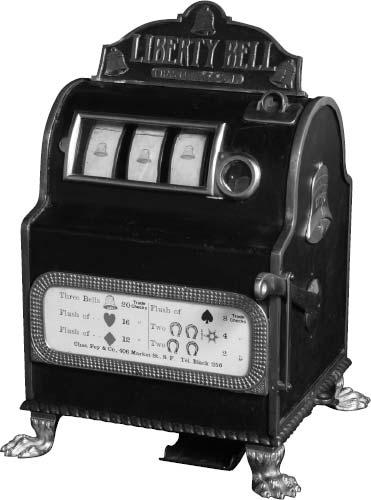
The size of a cash register, Charles Fey’s Liberty Bell was an immediate success when it was first manufactured at the very end of the nineteenth century.
Baerlocher and I met at IGT’s head office in a Reno business park, a 20-minute drive from the Peppermill Casino. He walked me through the production line, where tens of thousands of slot machines are built every year, and past a storage hall where hundreds were neatly stacked in rows. Baerlocher was clean-shaven and preppy, with short dark hair and a dimple in his chin. Originally from Carson City, half an hour’s drive away, he joined IGT after completing a maths degree at Notre Dame University, Indiana. For someone who loved inventing games as a child, and discovered a talent for probability at college, the job was a perfect fit.
When I wrote earlier that the core concept of gambling was the notion of expected value, I was giving only half the story. The other half is what mathematicians call the law of large numbers. If you bet only a few times on roulette or on the slots, you might come out on top. The more you play roulette, however, the more likely it is that you will lose overall. Payback percentages are only true in the long run.
The law of large numbers says that if a coin is flipped three times, it might not come up heads at all, but flip it three billion times and you can be pretty sure that it wil come up heads almost exactly 50 percent of the time. During the Second World War, the mathematician John Kerrich was visiting Denmark when he was arrested and interned by the Germans. With time on his hands, he decided to test the law of large numbers and flipped a coin 10,000 times in his prison cell. The result: 5067 heads, or 50.67 percent of the total. Around 1900, the statistician Karl Pearson did the same thing 24,000 times. With significantly more trials, you would expect the percentage to be closer to 50 percent – and it was. He threw 12,012 heads, or 50.05 percent.
The results mentioned above seem to confirm
what we take for granted – that in a coin flip the outcome of heads
is equally likely as the outcome of tails. Recently, however, a
team at Stanford University led by the statistician Persi Diaconis
investigated whether heads really are as likely to show up as
tails. The team built a coin-tossing machine and took slow-motion
photography of coins as they spun through the air. After pages of
analysis, including estimates that a nickel will land on its edge
in about 1 in 6000 throws, Diaconis’s results appeared to show the
fascinating and surprising result that a coin will, in fact, land
on the same face from which it was launched about 51 percent of the
time. So, if a coin is launched heads up, it will land on heads
slightly more often than it will land on tails. Diaconis concluded,
though, that what his research really proved was how difficult it
is to study random phenomena and that ‘for tossed coins, the
classical assumptions of independence with probability are pretty
solid’.
Casinos are all about large numbers. As Baerlocher explained, ‘Instead of just having one machine [casinos] want to have thousands because they know if they get the volume, even though one machine maybe what we call “upside-down” or losing, the group as a collective has a very strong probability of being positive for them.’ IGT’s slots are designed so that the payback percentage is met, within an error of 0.5 percent, after ten million games. At the Peppermill, where I was staying during my visit to Reno, each machine racks up about 2000 games a day. With almost 2000 machines, this makes a daily casino rate of four million games a day. After two and a half days, the Peppermill can be almost certain that it will be hitting its payback percentage within half a percent. If the average bet is a dollar, and the percentage is set to 95 percent, this works out to be $500,000 in profit, give or take $50,000, every 60 hours. It is little wonder, then, that slots are increasingly favoured by casinos.
The rules of roulette and craps haven’t changed since the games were invented centuries ago. By contrast, part of the fun of Baerlocher’s job is that he gets to devise new sets of probabilities for each new slot machine that IGT introduces to the market. First, he decides what symbols to use on the reel. Traditionally, they are cherries and bars, but they are now as likely to be cartoon characters, Renaissance painters, or animals. Then he works out how often these symbols are on the reel, what combinations result in payouts, and how much the machine pays out per winning combination.
Baerlocher drew me up a simple game, Game A
opposite, which has three reels and 82 positions per reel made up
of cherries, bars, red sevens, a jackpot and blanks. If you read
the table, you can see that there is a  or 10.976 percent chance of
cherry coming up on the first reel, and when this happens $1 wins a
$4 payout. The probability of a winning combination multiplied by
the payout is called the expected
contribution. The expected contribution of
cherry-aning-anything is 4×10.967 = 43.902 percent. In other words,
for every $1 put into the machine, 43.902 cents will be paid out on
cherry-anything-anything. When he is designing games, Baerlocher
needs to make sure the sum of expected contributions for all
payouts equals the desired payback percentage of the whole
machine.
or 10.976 percent chance of
cherry coming up on the first reel, and when this happens $1 wins a
$4 payout. The probability of a winning combination multiplied by
the payout is called the expected
contribution. The expected contribution of
cherry-aning-anything is 4×10.967 = 43.902 percent. In other words,
for every $1 put into the machine, 43.902 cents will be paid out on
cherry-anything-anything. When he is designing games, Baerlocher
needs to make sure the sum of expected contributions for all
payouts equals the desired payback percentage of the whole
machine.
The flexibility of slot design is that you can vary the symbols, the winning combinations and the payouts to make very different games. Game A is a ‘cherry dribbler’ – a machine that pays out frequently, but in small amounts. Almost half of the total payout money is accounted for in payouts of just $4. By contrast, in Game B only a third of the payout money goes on $4 payouts, leaving much more money to be won in the larger jackpots. Game A is what is called a low-volatility game, while Game B is high-volatility – you hit a winning combination less often, but the chances of a big win are greater. The higher the volatility, the more short-term risk there is for the slot operator.
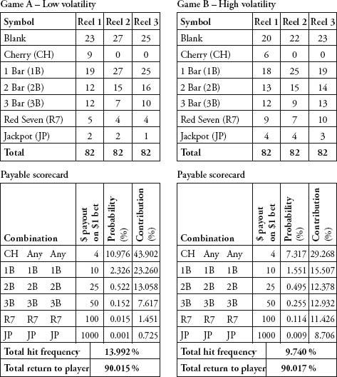
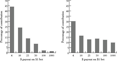
Some gamblers prefer low-volatility slots, while others prefer high. The game designer’s chief role is to make sure the machine pays out just enough for the gambler to want to continue playing – because the more someone plays, on average, the more he or she will lose. High volatility generates more excitement – especially in a casino, where machines hitting jackpots draw attention by erupting in spine-tingling son et lumière. Designing a good game, however, is not just about sophisticated graphics, colourful sounds and entertaining video narratives – it’s also about getting the underlying probabilities just right. I asked Baerlocher whether by playing around with volatility it was possible to design a low-payback machine that was more attractive to gamblers than a higher-payback machine. ‘My colleague and I spent over a year mapping things out and writing down some formulas and we came up with a method of hiding what the true payback percentage is,’ he said. ‘We’re now hearing from some casinos that they are running lower-payback machines and that the players can’t really pick up on it. It was a big challenge.’
I asked if this wasn’t a touch unethical.
‘It’s something that’s necessary,’ he replied. ‘We want the players to still enjoy it but we need to make sure that our customers make money.’
Baerlocher’s pay tables are helpful not just in order to understand the inner constitutions of one-armed bandits; they are also illustrative in explaining how the insurance industry works. Insurance is very much like playing the slots. Both are systems built on probability theory in which the losses of almost everyone pay for the winnings of a few. And both can be fantastically profitable for those controlling the payback percentages.
An insurance premium is no different from a gamble. You are betting on the chance that, for example, your house will be burgled. If your house is burgled, you receive a payout, which is the reimbursement for what was stolen. If your house isn’t burgled you, of course, receive nothing. The actuary at the insurance company behaves exactly like Anthony Baerlocher at IGT. He knows how much he wants to pay back to customers overall. He knows the probability for each payout event (a burglary, a fire, serious illness, etc.), so he works out how much his payouts should be per event so that the sum of expected contributions equals the total payback amount. Although compiling insurance tables is vastly more complicated than creating slot machines, the principle is the same. Since insurance companies pay out less than they receive in premiums, their payout percentage is less than 100 percent. Buying an insurance policy is a negative-expectation bet and, as such, it is a bad gamble.
So why do people take out insurance if it’s such a bad deal? The difference between insurance and gambling in casinos is that in casinos you are (hopefully) gambling with money you can afford to lose. With insurance, however, you are gambling to protect something you cannot afford to lose. While you will inevitably lose small amounts of money (the premium), this guards you against losing a catastrophic amount of money (the value of the contents of your house, for example). Insurance offers a good price for peace of mind.
It follows, however, that insuring against losing a non-catastrophic amount of money is pointless. One example is insuring against loss of a mobile phone. Mobile phones are relatively cheap (say, £100), but phone insurance is expensive (say, £7 per month). On average you will be better off if you don’t take out insurance, and instead buy yourself a new phone on the occasions that you lose it. In this way, you are ‘self-insuring’ and keeping the insurance company’s profit margins for yourself.
One reason for recent growth in the slots market is the introduction of ‘progressive’ machines, which have little to do with enlightened social policy and lots to do with the dream of instant wealth. Progressive slots have higher jackpots than other machines because they are joined in a network, with each machine contributing a percentage to a communal jackpot, the value of which gets progressively larger. In the Peppermill I had been struck by rows of linked machines offering prizes in the tens of thousands of dollars.
Progressive machines have high volatility, which means that in the short term casinos can lose significant sums. ‘If we put out a game with a progressive jackpot, about one in every twenty [casino owners] will write us a letter telling us our game is broken. Because this thing hit two or three jackpots in the first week and the machines are $10,000 in the hole,’ Baerlocher said, finding it ironic that people who are trying to profit from probability still have trouble understanding it on a basic level. ‘We’ll do an analysis and see the probability of it happening is, say, 200 to 1. They had [results] that should only happen half of a percent of the time – it had to happen to someone. We tell them, ride it out, it’s normal.’
IGT’s most popular progressive slot, Megabucks, links together hundreds of machines across Nevada. When the company introduced it a decade ago, the minimum jackpot was $1 million. Initially, casinos didn’t want the liability of having to pay out so much, so IGT underwrote the entire network by taking a percentage from all of its machines, and paid the jackpot itself. Despite paying out hundreds of millions of dollars in prize money, IGT has never suffered a loss on Megabucks. The law of large numbers is remarkably reliable: the bigger you get, the better it all works out.
The Megabucks jackpot now starts at $10 million. If it hasn’t been won by the time the jackpot reaches around $20 million, casinos see queues forming at their Megabucks slots and IGT gets requests to distribute more machines. ‘People think it’s past that point where i normally hits so it’s going to hit soon,’ explained Baerlocher.
This reasoning, however, is erroneous. Every game played on a slot machine is a random event. You are just as likely to win when the jackpot is at $10, $20 or even $100 million, but it is very instinctive to feel that after a long period of holding money back, the machines are more likely to pay out. The belief that a jackpot is ‘due’ is known as the gambler’s fallacy.
The gambler’s fallacy is an incredibly strong human urge. Slot machines tap into it with particular virulence, which makes them, perhaps, the most addictive of all casino games. If you are playing many games in quick succession, it is only natural to think after a long run of losses: ‘I’m bound to win next time.’ Gamblers often talk of a machine being ‘hot’ or ‘cold’ – meaning that it is paying out lots or paying out little. Again, this is nonsense, since the odds are always the same. Still, one can see why one might attribute personality to a human-sized piece of plastic and metal often referred to as a one-armed bandit. Playing a slot machine is an intense, intimate experience – you get right up close, tap it with your fingertips, and cut out the rest of the world.
Because our brains are bad at understanding randomness, probability is the branch of maths most riddled with paradoxes and surprises. We instinctively attribute patterns to situations, even when we know there are none. It’s easy to be dismissive of a slot-machine player for thinking that a machine is more likely to pay out after a losing streak, yet the psychology of the gambler’s fallacy is present in non-gamblers too.
Consider the following party trick. Take two people, and explain to them that one will flip a coin 30 times and write down the order of heads and tails. The other will imagine flipping a coin 30 times, and then will write down the order of heads and tails outcomes that they have visualized. Without telling you, the two players will decide who takes which role, and then present you with their two lists. I asked my mother and stepfather to do this and was handed the following:
List 1
H T T H T H T T T H H T H H T H H H H T H T T H T H T T H H
List 2
T T H H T T T T T H H T T T H T T H T H H H H T H H T H T H
The point of this game is that it is very easy to spot which list comes from the flipping of the real coin, and which from the imagined coin. In the above case, it was clear to me that the second list was the real one, which was correct. First, I looked at the maximum runs of heads or tails. The second list had a maximum run of 5 tails. The first list had a maximum run of 4 heads. The probability of a run of 5 in 30 flips is almost two thirds, so it is much more likely than not that 30 flips gives a run of 5. The second list was already a good candidate for the real coin. Also, I knew that most people never ascribe a run of 5 in 30 flips because it seems too deliberate to be random. But to be sure I was right that the second list was the real coin I looked at how frequently both lists alternated between heads and tails. Due to the fact that each time you flip a coin the chances of heads and tails are equal, you would expect each outcome to be followed by a different outcome about half the time, and half the time to be followed by the same outcome. The second list alternates 15 times. The first list alternates 19 times – evidence of human interference. When imagining coin flips, our brains tend to alternate outcomes much more frequently than what actually occurs in a truly random sequence – after a couple of heads, our instinct is to compensate and imagine an outcome of tails, even though the chance of heads is still just as likely. Here, the gambler’s fallacy appears. True randomness has no memory of what came before.
The human brain finds it incredibly difficult, if not impossible, to fake randomness. And when we are presented with randomness, we often interpret it as non-random. For example, the shuffle feature on an iPod plays songs in a random order. But when Apple launched the feature, customers complained that it favoured certain bands because often tracks from the same band were played one after another. The listeners were guilty of the gambler’s fallacy. If the iPod shuffle were truly random, then each new song choice is independent of the previous choice. As the coin-flipping experiment shows, counterintuitively long streaks are the norm. If songs are chosen randomly, it is very possible, if not entirely likely, that there will be clusters of songs by the same artist. Apple CEO Steve Jobs was totally serious when he said, in response to the outcry: ‘We’re making [the shuffle] less random to make it feel more random.’
Why is the gambler’s fallacy such a strong human urge? It’s all about control. We like to feel in control of our environments. If events occur randomly, we feel that we have no control over them. Conversely, if we do have control over events, they are not random. This is why we prefer to see patterns when there are none. We are trying to salvage a feeling of control. The human need to be in control is a deep-rooted survival instinct. In the 1970s a fascinating (if brutal) experiment examined how important a sense of control was for elderly patients in a nursing home. Some patients were allowed to choose how their rooms were arranged and allowed to choose a plant to look after. The others were told how their rooms would be and had a plant chosen and tended for them. The result after 18 months was striking. The patients who had control over their rooms had a 15 percent death rate, but for those who had no control the rate was 30 percent. Feeling in control can keep us alive.
Randomness is not smooth. It creates areas of empty space and areas of overlap.
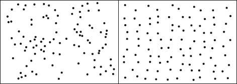
Random dots; non-random dots.
Randomness can explain why some small villages have higher than normal rates of birth defects, why certain roads have more accidents, and why in some games basketball players seem to score every free throw. It’s also why in seven of the last ten World Cup finals at least two players shared birthdays:
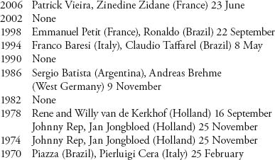
While at first this seems like an amazing series of coincidences, the list is actually mathematically unsurprising because whenever you have a randomly selected group of 23 people (such as two football teams and a referee), it is more likely than not that two people in it will share the same birthday. The phenomenon is known as the ‘birthday paradox’. There is nothing self-contradictory about the result, but it does fly in the face of common sense – twenty-three seems like an absurdly small number.
Proof of the birthday paradox is similar to the proofs we used at the beginning of this chapter for rolling certain combinations of dice. In fact, we could rephrase the birthday paradox as the statement that for a 365-sided dice, after 23 throws it will be more likely than not that the dice will have landed on the same side twice.
Step 1: The probability of two people sharing the same birthday in a group is 1 minus the probability of no one sharing the same birthday.
Step 2: The probability of no one sharing the same birthday in a group of two people is
. This is because the first person can be born on any day (365 choices out of 365) and the second can be born on any day apart from the day the first one is (364 choices out of 365). For convenience, we will ignore the extra day in a leap year.
Step 3: The probability of no one sharing the same birthday in a group of three people is
. With four people it becomes
, and so on. When you multiply this out the result gets smaller and smaller. When the group contains 23 people, it finally shrinks to below 0.5 (the exact number is 0.493).
Step 4: If the probability of no one sharing the same birthday in a group is less than 0.5, the probability of at least two people sharing the same birthday is more than 0.5 (from Step 1). So it is more likely than not that in a group of 23 people two will have been born on the same day.
Football matches provide the perfect sample group to see if the facts fit the theory because there are always 23 people on the pitch. Looking at World Cup finals, however, the birthday paradox works a little too well. The probability of two people having the same birthday in a group of 23 is 0.507 or just over 50 percent. Yet with seven out of ten positives (even excluding the van de Kerkhof twins), we have achieved a 70 percent strike rate.
Part of this is the law of large numbers. If I analysed every match in every World Cup, I can be very confident that the result would be closer to 50.7 percent. Yet there is another variable. Are the birthdays of footballers equally distributed throughout the year? Probably not. Research shows that footballers are more likely to be born at certain times of the year – favouring those born just after the school year cut-off point, since they will be the oldest and largest in their school years, and will therefore dominate sports. If there is a bias in the spread of birth dates, we can expect a higher chance of shared birthdays. And often there is a bias. For example, a sizeable proportion of babies are now born by caesarian section or induced. This tends to happen on weekdays (as maternity staff prefer not to work weekends), with the result that births are not spread as randomly throughout the year. If you take a section of 23 people born in the same 12-month period – say, the children in a primary-school classroom – the chance of two pupils sharing the same birthday will be significantly more than 50.7 percent.
If a group of 23 people is not immediately accessible to test this out, just look at your immediate family. With 4 people it is 70 percent likely that 2 will have birthdays within the same month. You y need 7 people for it to be likely that 2 of them were born in the same week, and in a group of 14 it is as likely as not that 2 people were born within a day of each other. As group size gets bigger, the probability rises surprisingly fast. In a group of 35 people, the chance of a shared birthday is 85 percent, and with a group of 60 the chance is more than 99 percent.
Here’s a different question about birthdays with an answer as counter-intuitive as the birthday paradox: how many people do there need to be in a group for there to be a more than 50 percent chance that someone shares your birthday. This is different from the birthday paradox because we are specifying a date. In the birthday paradox we are not bothered who shares a birthday with whom; we just want a shared birthday. Our new question can be rephrased as: given a fixed date, how many times do we need to roll our 365-sided dice until it lands on this date? The answer is 253 times! In other words, you would need to assemble a group of 253 people just to be more sure than not that one of them shares your birthday. This seems absurdly large – it is well over halfway between one and 365. Yet randomness is doing its clustering thing again – the group needs to be that size because the birthdays of its members are not falling in an orderly way. Among those 253 people there will be many people who double up on birthdays that are not yours, and you need to take them into account.
A lesson of the birthday paradox is that coincidences are more common than you think. In German Lotto, like the UK National Lottery, each combination of numbers has a 1-in-14-million chance of winning. Yet in 1995 and in 1986 identical combinations won: 15-25-27-30-42-48. Was this an amazing coincidence? Not especially, as it happens. Between the two occurrences of the winning combination there were 3016 lottery draws. The calculation to find how many times the draw should pick the same combination is equivalent to calculating the chances of two people sharing the same birthday in a group of 3016 people with there being 14 million possible birthdays. The probability works out to be 0.28. In other words, there was more than a 25 percent chance that two winning combinations would be identical over that period; so the ‘coincidence’ was therefore not an extremely weird occurrence.
More disturbingly, a misunderstanding of
coincidence has resulted in several miscarriages of justice. In one
famous California case, from 1964, witnesses to a mugging reported
seeing a blonde with a ponytail, a black man with a beard and a
yellow getaway car. A couple fitting this description were arrested
and charged. The prosecutor calculated the chance of such a couple
existing by multiplying the probabilities of the occurrence of each
of detail together:  for a yellow car,
  for a blonde, and so on. The
prosecutor calculated that the chance of such a couple existing was
1 in 12 million. In other words, for every 12 million people, only
one couple on average would fit the exact description. The chances
of the arrested couple being the guilty couple, he argued, were
overwhelming. The couple was convicted.
for a blonde, and so on. The
prosecutor calculated that the chance of such a couple existing was
1 in 12 million. In other words, for every 12 million people, only
one couple on average would fit the exact description. The chances
of the arrested couple being the guilty couple, he argued, were
overwhelming. The couple was convicted.
The prosecutor, however, was doing the wrong calculation. He had worked out the chance of randomly selecting a couple that matched the witness profiles. The relevant question should have been, given there is a couple that matches the description, what is the chance that the arrested couple is the guilty couple? This probability was only about 40 percent. More likely than not, therefore, the fact that the arrested couple fitted the description was a coincidence. In 1968 the California Supreme Court reversed the conviction.
Returning to the world of gambling, in another lottery case a New Jersey woman won her state lottery twice in four months in 1985–6. It was widely reported that the chances of this happening was 1 in 17 trillion. However, though 1 in 17 trillion was the correct chance of buying a single lottery ticket in both lotteries and scooping the jackpot on both occasions, this did not mean that the chances of someone, somewhere winning two lotteries was just as unlikely. In fact, it is pretty likely. Stephen Samuels and George McCabe of Purdue University calculated that over a seven-year period the odds of a lottery double-win in the United States are better than evens. Even over a four-month period, the odds of a double winner somewhere in the country are better than 1 in 30. Persi Diaconis and Frederick Mosteller call this the law of very large numbers: ‘With a large enough sample, any outrageous thing is apt to happen.’
Mathematically speaking, lotteries are by far the worst type of legal bet. Even the most miserly slot machine has a payback percentage of about 85 percent. By comparison, the UK National Lottery has a payback percentage of approximately 50 percent. Lotteries offer no risk to the organizers since the prize money is just the takings redistributed. Or, in the case of the National Lottery, half of the takings, redistributed.
In rare instances, however, lotteries can be the best bet around. This is the case when, due to ‘rollover’ jackpots, the prize money has grown to become larger than the cost of buying every possible combination of numbers. In these instances, since you are covering all outcomes, you can be assured of having the winning combination. The risk here is only that there might be other people who also have the winning combination – in which case you will have to share the first prize with them. The buy-every-combination approach, however, relies on an ability to do just that – which is a significant theoretical and logistical challenge.
The UK lottery is a 6/49 lottery, which means that for each ticket the punter must select 6 numbers out of 49. There are about 14 million possible combinations. How do you list these combinations in such a way that each combination is listed exactly once, avoiding duplications? In the early 1960s, Stefan Mandel, a Romanian economist, asked himself the same question about the smaller Romanian lottery. The answer is not straightforward. Mandel cracked it, however, after spending several years on the problem and won the Romanian lottery in 1964. (In fact, in this case he did not buy every combination, since that would have cost him too much money. He used a supplementary method called ‘condensing’ that guarantees that at least 5 of the 6 numbers are correct. Usually getting 5 numbers means winning second prize, but he was lucky and won first prize first time.) The algorithm that Mandel had written out to decide which combinations to buy covered 8000 foolscap sheets. Shortly afterwards, he emigrated to Israel and then to Australia.
While in Melbourne, Mandel founded an international betting syndicate, raising enough money from its members to ensure that, if he wanted to buy every single combination in a lottery, then he could. He surveyed the world’s lotteries for rollover jackpots that were more than three times the cost of every combination. In 1992 he identified the Virginia state lottery – a lottery with seven million combinations, each costing $1 a ticket – whose jackpot had reached almost $28 million. Mandel got to work. He printed out coupons in Australia, filled them in by computer so that they covered the seven million combinations, and then flew the coupons to the UShad w won the first prize and 135,000 secondary prizes too.
The Virginia lottery was Mandel’s largest jackpot, bringing his tally since leaving Romania to 13 lottery wins. The US Internal Revenue Service, the FBI and the CIA all looked into the syndicate’s Virginia lottery win, but could prove no wrongdoing. There is nothing illegal about buying up every combination, even though it sounds like a scam. Mandel has now retired from betting on lotteries and lives on a tropical island in the South Pacific.
A particularly useful visualization of randomness was invented by John Venn in 1888. Venn is perhaps the least spectacular mathematician ever to become a household name. A Cambridge professor and Anglican cleric, he spent much of his later life compiling a biographical register of 136,000 of the university’s pre-1900 alumni. While he did not push forward the boundaries of his subject, he did, nevertheless, develop a lovely way of explaining logical arguments with intersecting circles. Even though Leibniz and Euler had both done something very similar in previous centuries, the diagrams are named after Venn. Much less known is that Venn thought up an equally irresistible way to illustrate randomness.
Imagine a dot in the middle of a blank page. From the dot there are eight possible directions to go: north, northeast, east, southeast, south, southwest, west and northwest. Assign the numbers 0 to 7 to each of the directions. Choose a number from 0 to 7 randomly. If the number comes up, trace a line in that direction. Do this repeatedly to create a path. Venn carried this out with the most unpredictable sequence of numbers he knew: the decimal expansion of pi (excluding 8s and 9s, and starting with 1415). The result, he wrote, was ‘a very fair graphical indication of randomness’.
Venn’s sketch is thought to be the first-ever diagram of a ‘random walk’. It is often called the ‘drunkard’s walk’ because it is more colourful to imagine that the original dot is instead a lamp-post and the path traced is the random staggering of a drunk. One of the most obvious questions to ask is how far will the drunk wander from the point of origin before collapsing? On average, the longer he has been walking, the further away he will be. It turns out that his distance increases with the square root of the time spent walking. So, if in one hour he stumbles, on average, one block from the lamp-post, it will take him four hours, on average, to go two blocks, and nine hours to go three.
As the drunkard randomly walks, there will be times when he goes in circles and doubles back on himself. What is the chance of the drunk eventually walking back into the lamp-post? Surprisingly, the answer is 100 percent. He might stray for years in the most remote places but it is a sure thing that, given sufficient time, the drunk will eventually return to base.
Imagine a drunkard’s walk in three dimensions. Call it the buzz of the befuddled bee. The bee starts at a point suspended in space and then flies in a straight line in a random direction for a fixed distance. The bee stops, dozes, then buzzes off in another random direction for the same distance. And so on. What is the chance of the bee eventually buzzing back into the spot where it started? The answer is only 0.34, or about a third. It was weird to realize that in two dimensions the chance of a drunkard walking back into the lamp-post was an absolute certainty, but it seems even weirder to think that a bee buzzing for ever is very unlikely ever to return home.
The first-ever random walk appeared in the third edition of John Venn’s Logic of Chance (1888). The rules for the direction of the walk (my addition) follow the digits 0–7 that appear in pi after the decimal point.
In Luke Rhinehart’s bestselling novel The Dice Man, the eponymous hero makes life decisions based on the throwing of dice. Consider Coin Man, who makes decisions based on the flip of a coin. Let’s say that if he flips heads, he moves one step up the page, and if he flips tails, he moves a step down the page. Coin Man’s path is a drunkard’s walk in one dimension – he can move only up and down the same line. Plotting the walk described by the second list of 30 coin flips chapter 9, you get the following graph.
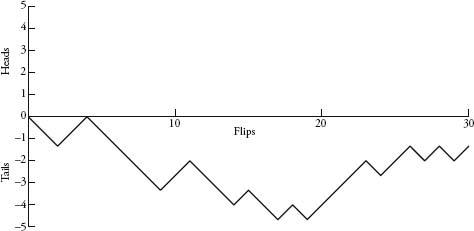
The walk is a jagged line of peaks and valleys. If you extended this for more and more flips, a trend emerges. The line swings up and down, with larger and larger swings. Coin Man roams further and further from his starting point in both directions. Below are the journeys of six coin men that I plotted from 100 flips each.

If we imagine that at a certain distance from the starting point in one direction there is a barrier, there is a 100 percent probability that eventually Coin Man will hit the barrier. The inevitability of this collision is very instructive when we analyse gambling patterns.
Instead of letting Coin Man’s random walk describe a physical journey, let it represent the value of his bank account. And let the coin flip be a gamble. Heads he wins £100, tails he loses £100. The value in his bank account will swing up and down in increasingly large waves. Let us say that the only barrier that will stop Coin Man playing is when the value of his account is £0. We know it is guaranteed he will get there. In other words, he will always go bankrupt. This phenomenon – that eventual impoverishment is a certainty – is known evocatively as gambler’s ruin.
Of course, no casino bets are as generous as the flipping of a coin (which has a payback percentage of 100). If the chances of losing are greater than the chances of winning, the map of the random walk drifts downward, rather than tracking the horizontal axis. In other words, bankruptcy looms quicker.
Random walks explain why gambling favours the very rich. Not only will it take much longer to go bankrupt, but there is also more chance that your random walk will occasionally meander upward. The secret of winning, for the rich or the poor, however, is knowing when to stop.
Inevitably, the mathematics of random walks contains some head-popping paradoxes. In the graphs chapter 9 where Coin Man moves up or down depending on the results of a coin toss, one would expect the graph of his random walk to regularly cross the horizontal axis. The coin gives a 50:50 chance of heads or tails, so perhaps we would expect him to spend an equal amount of time either side of his starting point. In fact, though, the opposite is true. If the coin is tossed infinitely many times, the most likely number of times he will swap sides is zero. The next most likely number is one, then two, three and so on.
For finite numbers of tosses there are still some pretty odd results. William Feller calculated that if a coin is tossed every second for a year, there is a 1-in-20 chance that Coin Man will be on one side of the graph for more than 364 days and 10 hours. ‘Few people believe that a perfect coin will produce preposterous sequences in which no change of [side] occurs for millions of trials in succession, and yet this is what a good coin will do rather regularly,’ he wrote in An Introduction to Probability Theory and Its Applications. ‘If a modern educator or psychologist were to describe the long-run case histories of individual coin-tossing games, he would classify the majority of coins as maladjusted.’
While the wonderful counter-intuitions of randomness are exhilarating to pure mathematicians, they are also alluring to the dishonourable. Lack of a grasp of basic probability means that you can easily be conned. If you are ever tempted, for example, by a company that claims it can predict the sex of your baby, you are about to fall victim to one of the oldest scams in the book. Imagine I set up a company, which I’ll call BabyPredictor, that announces a scientific formula for predicting whether a baby will be a boy or a girl. BabyPredictor charges mothers a set fee for the prediction. Because of a formidable confidence in its formula, and the philanthropic generosity of its CEO, me, the company also offers a total refund if the prediction turns out to be wrong. Buying the prediction sounds like a good deal – since either BabyPredictor is correct, or it is wrong and you can get your money back. Unfortunately, however, BabyPredictor’s secret formula is actually the tossing of a coin. Heads I say the child will be a boy, tails it will be a girl. Probability tells me that I will be correct about half the time, since the ratio of boys to girls is about 50:50. Of course, half the time I will give the money back, but so what – since the other half of the time I get to keep it.
The scam works because the mother is unaware of the big picture. She sees herself as a sample group of one, rather than as part of a larger whole. Still, baby-predicting companies are alive and well. Babies are born every minute, and so are mugs.
In a more elaborate version, this time targeting greedy men rather than pregnant women, a company we’ll call StockPredictor puts up a fancy website. It sends out 32,000 emails to an investors’ mailing list, announcing a new service, which, using a very sophisticated computer model, can predict whether a certain stock index will rise or fall. In half of the emails it predicts a rise the following week; and in the other half, a fall. Whatever happens to the index, 16,000 investors will have received an email with the correct prediction. So, StockPredictor then sends these 16,000 addresses another email with the following week’s prediction. Again, the prediction will be correct for 8000 of them. If StockPredictor continues like this for another four weeks, eventually there will be 1000 email recipients whose six consecutive predictions have all turned out to be true. StockPredictor then informs them that in order to receive any further predictions they must pay a fee – and why wouldn’t they, since the predictions have thus far been pretty good?
The stock-predicting scam can be adapted to predicting horse-races, football matches, and even the weather. If all outcomes are covered, there will be at least one person receiving a correct prediction of all matches, races or sunny days. That person might think, ‘Wow, there is only a one-in-a-million chance of such a combination being true,’ but if a million emails are sent out covering all possibilities, then someone, somewhere has to receive the correct one.
Scamming people is immoral and often illegal. However, trying to get one over on a casino is often seen as a just cause. For mathematicians, the challenge of beating the odds is like showing a red rag to a bull – and there is an honourable tradition of those who have succeeded.
The first method of attack is to realize that the world is not perfect. Joseph Jagger was a cotton-factory mechanic from Lancashire who knew enough about Victorian engineering to realize that roulette wheels might not spin perfectly true. His hunch was that if the wheel was not perfectly aligned, it might favour some numbers over others. In 1873, aged 43, he visited Monte Carlo to test his theory. Jagger hired six assistants, assigned each of them to one of the six tables in a casino, and instructed them to write down every number that came up over a week. Upon analysing the figures, he saw that one wheel was indeed biased – nine numbers came up more than others. The greater prevalence of these numbers was so slight that their advantage was only noticeable when considering hundreds of plays.
Jagger started betting and in one day won the equivalent of $70,000. Casino bosses, however, noticed that he gambled at only one table. To counter Jagger’s onslaught, they switched the wheels around. Jagger started to lose, until he realized what the management had done. He relocated to the biased table, which he recognized because it had a distinctive scratch. He started winning again and only gave up when the casino reacted a second time by sliding the frets around the wheel after each daily session, so that new numbers would be favoured. By that time Jagger had already amassed $325,000 – making him, in today’s terms, a multimillionaire. He returned home, left his factory job and invested in real estate. In Nevada, from 1949 to 1950, Jagger’s method was repeated by two science grads named Al Hibbs and Roy Walford. They started off with a borrowed $200 and turned it into $42,000, allowing them to buy a 40ft yacht and sail the Caribbean for 18 months before returning to their studies. Casinos now change wheels around much more regularly than they used to.
The second way to manipulate the odds in your favour is to question what randomness is anyway. Events that are random under one set of information might well become non-random under a greater set of information. This is turning a maths problem into a physics one. A coin flip is random because we don’t know how it will land, but flipped coins obey Newtonian laws of motion. If we knew exactly the speed and angle of the flip, the density of the air and any other relevant physical data, we would be able to calculate exactly the face on which it would land. In the mid 1950s a young mathematician named Ed Thorp began to ponder what set of information would be required to predict where a ball would land in roulette.
Thorp was helped in his endeavour by Claude Shannon, his colleague at the Massachusetts Institute of Technology. He couldn’t have wished for a better co-conspirator. Shannon was a prolific inventor with a garage full of electronic and mechanical gadgets. He was also one of the most important mathematicians in the world, as the father of information theory, a crucial academic breakthrough that led to the development of the computer. The men bought a roulette wheel and conducted experiments in Shannon’s basement. They discovered that if they knew the speed of the ball as it went around the stationary outer rim, and the speed of the inner wheel (which is spun in the opposite direction of the ball), they could make pretty good estimates regarding which segment of the wheel the ball would fall in. Since casinos allow players to place a bet after the ball has been dropped, all Thorp hannon needed to do was figure out how to measure the speeds and process them in the few seconds before the croupier closed the betting.
Once again, gambling pushed forward scientific advancement. In order to predict roulette plays accurately, the mathematicians built the world’s first wearable computer. The machine, which could fit in a pocket, had a wire going down to the shoe, where there was a switch, and another wire going up to a pea-sized headphone. The wearer was required to touch the switch at four moments – when a point on the wheel passed a reference point, when it had made one full revolution, when the ball passed the same point, and when the ball had again made a full revolution. This was enough information for estimating the speeds of the wheel and the ball.
Thorp and Shannon divided the wheel into eight segments of five numbers each (some overlapped, though, as there are 38 pockets). The pocket-sized computer played a scale of eight notes – an octave – through the headphones and the note it stopped on determined the segment where it predicted the ball would fall. The computer could not say with total certainty which segment the ball would land in, but it didn’t need to. All Thorp and Shannon desired was that the prediction would be better than the randomness of guessing. On hearing the notes, the computer-wearer would then place chips on all five numbers of the segment (which, although next to each other on the wheel, were not adjacent on the baize). The method was surprisingly accurate – for the single-number bets they estimated that they could expect to win $4.40 for every $10 wager.
When Thorp and Shannon went to Las Vegas for a test drive, the computer worked, if precariously so. The men needed to look inconspicuous, but the earpiece was prone to popping out and the wires were so fragile that they kept breaking. Still, the system worked, and they were able to convert a small pile of dimes into a few piles of dimes. Thorp was content to have beaten roulette in theory, if not in practice, because his assault on another gambling game was having much more striking success.
Blackjack, or twenty-one, is a card game in which the aim is to get a hand where the total value of the cards is as close as possible to an upper limit of 21. The dealer also deals a hand for himself. To win, you must have a hand higher than his while not exceeding 21.
Like all the classic casino games, blackjack gives a slight advantage to the house. If you play blackjack, in the long run you will lose money. In 1956 an article was published in an obscure statistics journal that claimed to have devised a playing strategy that gave the house an advantage of just 0.62 percent. After reading the article, Thorp learned the strategy and tested it during a vacation trip to Vegas. He discovered that he lost his money much slower than the other players. He decided he would begin to think deeply about blackjack, a decision that would change his life.
Ed Thorp is now 75 but I suspect he doesn’t look that different from how he looked half a century ago. Slim, with a long neck and concise features, he has a clean-cut college-boy haircut, unpretentious glasses, and a calm, upright posture. After returning from Vegas, Thorp reread the journal article. ‘I saw right away, within a couple of minutes, how you could almost certainly beat this game by keeping track of the cards that were played,’ he remembered. Blackjack is different from, say, roulette, since the odds change once a card has been dealt. The chance of getting a 7 in roulette is 1 in 38 every time you spin the wheel. In blackjack the probability>
 13. If the first dealt card is
an ace, the probability of the second card being an ace, however,
is not –
it is
13. If the first dealt card is
an ace, the probability of the second card being an ace, however,
is not –
it is  ,
since the pack now has 51 cards and there are only 3 aces left in
it. Thorp thought there must be a system that turned the odds in
the favour of the player. It then became just a matter of finding
it.
,
since the pack now has 51 cards and there are only 3 aces left in
it. Thorp thought there must be a system that turned the odds in
the favour of the player. It then became just a matter of finding
it.
In a 52-card deck there are 52×51×50×49×…×3×2×1 ways of the cards being ordered. This number is about 8×1067, or 8 followed by 67 zeros. The number is so huge that it is very unlikely that any two randomly shuffled decks will ever have had the same order in the history of the world – even if the world’s population had started playing cards at the Big Bang. Thorp reasoned that there are too many possible permutations of cards for any system of memorizing permutations to be feasible for a human brain. Instead he decided to look at how the house advantage changes depending on which cards have already been dealt. Using a very early computer, he found that by keeping track of the number-five cards of each suit – the five of hearts, spades, diamonds and clubs – a player could judge whether the deck was favourable. Under Thorp’s system, blackjack morphed into a beatable game, with an expected return of up to 5 percent depending on the cards left in the pack. Thorp had invented ‘card-counting’.
He wrote up his theory and submitted it to the American Mathematical Society (AMS). ‘When the abstract came through everybody thought it was ridiculous,’ he remembered. ‘It was gospel in the scientific world that you couldn’t beat any of the major gambling games, and that had rather strong support from the research and analysis that had been done over a couple of centuries.’ Proofs that demonstrate that you can beat the odds at casino games are rather like proofs that you can square the circle – surefire evidence of a crackpot. Luckily, one of the members of the AMS’s submission committee was an old classmate of Thorp’s, and the abstract was accepted.
In January 1961 Thorp presented his paper at the American Mathematical Society’s winter meeting in Washington. It made national news, including the front page of his local paper, the Boston Globe. Thorp received hundreds of letters and calls, with many offers to finance gambling sprees for a share of the profit. A syndicate from New York was offering $100,000. He called the number on the New York letter and the following month a Cadillac pulled up outside his apartment. Out stepped a pint-sized senior citizen, accompanied by two spectacular blondes in mink coats.
The man was Manny Kimmel, a mathematically astute New York gangster and inveterate high-stakes gambler. Kimmel had taught himself enough about probability to know the birthday paradox – one of his favourite things to bet on was whether two people in a group shared the same birthday. Kimmel introduced himself as the owner of 64 parking lots in New York City, which was true. He introduced the girls as his nieces, which probably wasn’t. I asked Thorp if he suspected Kimmel of mob ties. ‘At that time I wasn’t very knowledgeable about the gambling world; in fact I had no knowledge of it except the theoretical, and I also hadn’t investigated the world of crime. He represented himself as a wealthy businessman and the evidence for that was overwhelming.’ Kimmel invited Thorp to play blackjack at his luxurious Manhattan apartment the following we. After a few sessions, Kimmel was convinced that card-counting worked. Both men flew to Reno to try it out. They started off with $10,000 and by the end of the trip had built their pot up to $21,000.
When you are gambling in a casino, two factors come into play that determine how much money you will win or lose. Playing strategy is about how to win a game. Betting strategy is about money management – how much to bet and when. Is it worth, for example, betting your entire purse on one bet? Or is it worth dividing your money up into the smallest possible stakes? Different strategies can have a surprisingly large impact on how much money you can expect to make.
The best-known betting strategy is called the ‘martingale’, or doubling up, and was popular with French gamblers in the eighteenth century. The principle is to double your bet if you lose. Let’s say you are betting on the toss of a coin. Heads you win $1, tails you lose $1. Just say the first flip is tails. You lose $1. For the next bet you must stake $2. Winning on the second bet wins you $2, which recoups your $1 loss from the first bet and puts you $1 in profit. Say you lose the first five flips:
Lose $1 bet so next time bet $2
Lose $2 bet so next time bet $4
Lose $4 bet so next time bet £8
Lose $8 bet so next time bet $16
Lose $16 bet
You will be 1 + 2 + 4 + 8 + 16 = $31 down, so the sixth bet must be for $32. If you win you recoup your losses, and profit. But despite risking so much money, you are only ahead by $1, your original stake.
Martingale certainly has an appeal. In a game where the odds are almost 50:50 – like, say, betting on the red at roulette, which has a probability of 47 percent – you are very likely to win a fair percentage of plays and so have a good chance of staying ahead. But the martingale system is not fail-safe. For a start, you are only winning in small increments. And we know that in a run of 30 coin flips, a streak of five heads, or five tails, is more likely than not. If you start with a $40 bet and have a five-game losing streak, you will find yourself having to bet $1280. At the Peppermill Casino, though, you wouldn’t be able to – it has a maximum bet of $1000. One reason why casinos have maximum bets is to stop systems like martingale. The exponential growth of martingale bets on a losing streak often accelerates bankruptcy, rather than insuring against it. The system’s most famous champion, eighteenth-century Venetian playboy Giacomo Casanova, discovered this the hard way. ‘I still played on the martingale,’ he once said, ‘but with such bad luck that I was soon left without a sequin.’
Still, if you stood at the Peppermill roulette table playing martingale with a $10 starting stake on red, you would have to be very unlucky not to eventually win $10. The system would break down only if you lost six times in a row, and there is only a 1-in-47 chance of that happening. Once you have won, however, it would then be advisable to cash in your winnings and leave. By continuing to gamble, the chances of an unlucky streak will eventually become more likely than not.
Let’s consider a different system of betting. Imagine you are given $20,000 in a casino and told you must gamble it on red roulette table. What’s the best strategy for doubling your money? Is to be bold and bet the whole thing in one bet, or to be cautious and bet in the smallest possible amount, in stakes of $1? Even though it seems initially reckless, your chances of success are much better if you bet the whole amount in one go. In maths-speak, bold play is optimal. With a smidgen of reflection, this makes sense: the law of large numbers says that you will lose in the long run. Your best chances are to make the run as short as possible.
In fact, this is exactly what Ashley Revell, a 32-year-old from Kent, did in 2004. He sold all his possessions, including his clothes, and in a Las Vegas casino bet the total amount – $135,300 – on red. Had he lost, he would have at least become a C-list TV celebrity, as the bet was being filmed for a TV reality show. But the ball landed on red 7, and he came home with $270,600.
At blackjack, Ed Thorp was presented with a different issue. His card-counting system meant that he could tell at certain points during the game whether he had an advantage over the dealer. Thorp asked himself: what is the best betting strategy when the odds are in your favour?
Imagine there is a bet where the chance of winning is 55 percent and the chance of losing 45 percent. For simplicity, the game pays evens and we play it 500 times. The advantage – the edge – is 10 per cent. In the long run our winnings will work out on average as a $10 profit for every $100 gambled. To maximize our total profit, we obviously need to maximize the combined total of wagers. It is not immediately obvious how this is done, since maximizing wealth requires a minimizing of the risk of losing it all. This is how four betting strategies perform:
Strategy 1: Bet everything. Just like Ashley Revell, put your entire bankroll on the first bet. If you win, you have doubled your money. If you lose, you are bankrupt. If you win, put everything down again for the next bet. The only way you can avoid losing everything is if you win all 500 games. The chance of this happening, if the probability of winning each game is 0.55, is about one in 10130, or 1 followed by 130 zeros. In other words, it is almost certain you will be bankrupt by the 500th game. Obviously, this is not a good long-term strategy.
Stategy 2: Fixed wager. Bet a fixed amount on every bet. If you win, your wealth grows by that fixed amount. If you lose, your wealth shrinks by that amount. Since you win more than you lose, your wealth will increase overall, but it does so only by increasing in jumps of the same fixed amount. As the graph overleaf shows, your money doesn’t grow very fast.
Strategy 3: Martingale. This gives a faster rate than fixed wager, since losses are compensated by doubling up after a loss, but brings with it a much higher risk. With only a few losing bets, you could be bankrupt. Again, this is not a good long-term strategy.
Strategy 4: Proportional betting. In this case, bet a fraction of your bankroll related to the edge you have. There are several variations of proportional betting, but the system where wealth grows fastest is called the Kelly strategy. Kelly tells you to bet the f bankr your bankroll determined by
. In this case, the edge is 10 percent and the odds are evens (or 1 to 1), making
This is a very safe strategy because if you have a losing streak, the absolute value of the wager shrinks – which means that losses are limited. It also offers large potential rewards since – like compound interest – on a winning streak one’s wealth grows exponentially. It is the best of both worlds: low risk and high return. And just look how it performs: starting slowly but eventually, after around 400 bets, racing way beyond the others.
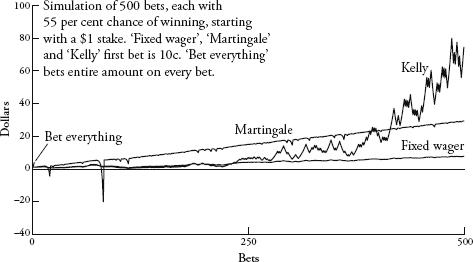
John Kelly Jr was a Texan mathematician who outlined his famous gambling strategy formula in a 1956 paper, and when Ed Thorp put it into practical use at the blackjack table, the results were striking. ‘As one general said, you get there firstest with the mostest.’ With small edges and judicious money management, huge returns could be achieved. I asked Thorp which method was more important to making money at blackjack – card-counting or using the Kelly criterion. ‘I think the consensus after decades of examining this question,’ he replied, ‘is that the betting strategies may be two thirds or three quarters of what you’re going to get out of it, and playing strategy is maybe a third to a quarter. So, the betting strategy is much more important.’ Kelly’s strategy would later help Thorp make more than $80 billion dollars on the financial markets.
Ed Thorp announced his card-counting system in his 1962 book Beat the Dealer. He refined the method for a second edition in 1966 that also counted the cards worth ten (the jack, queen, king and ten). Even though the ten cards shift the odds less than the five do, there are more of them, so it’s easier to identify advantages. Beat the Dealer sold more than a million copies, inspiring – and continuing to inspire – legions of gamblers.
In order to eliminate the threat of card-counting, casinos have tried various tactics. The most common was to introduce multiple decks because with more cards, counting is made both more difficult and less profitable. The ‘professor stopper’, a shoe that shuffles many packs at once, is essentially named in Thorp’s honour. And casinos have been forced to make it an offence to use a computer to predict at roulette.
Thorp last played blackjack in 1974. ‘The family went on a trip to the World’s Fair in Spokane and on the way back we stopped at Harrah’s [casino] and I told my kids to give me a couple of hours because I wanted to pay for the trip – which I did.’
Beat the Dealer is not just a gambling classic. It also reverberated through the worlds of economics and finance. A generation of mathematicians inspired by Thorp’s book began to create models of the financial markets and apply betting strategies to them. Two of them, Fischer Black and Myron Scholes, created the Black-Scholes formula indicating how to price financial derivatives – Wall Street’s most famous (and infamous) equation. Thorp ushered in an era when the quantitative analyst, the ‘quant’ – the name given to the mathematicians relied on by banks to find clever ways of investing – was king. ‘Beat the Dealer was kind of the first quant book out there and it led fairly directly to quite a revolution,’ said Thorp, who can claim – with some justification – to being the first-ever quant. His follow-up book, Beat the Market, helped transform securities markets. In the early 1970s he, together with a business partner, started the first ‘market neutral’ derivatives hedge fund, meaning that it avoided any market risk. Since then, Thorp has developed more and more mathematically sophisticated financial products, which has made him extremely rich (for a maths professor, anyway). Although he used to run a well-known hedge fund, he now runs a family office in which he invests only his own money.
I met Thorp in September 2008. We were sitting in his office in a high-rise tower in Newport Beach, which looks out over the Pacific Ocean. It was a delicious California day with a pristine blue sky. Thorp is scholarly without being earnest, careful and considered, but also sharp and playful. Just one week earlier, the bank Lehman Brothers had filed for bankruptcy. I asked him if he felt any sense of guilt for having helped create some of the mechanisms that had contributed to the largest financial crisis in decades. ‘The problem wasn’t the derivatives themselves, it was the lack of regulation of the derivatives,’ he replied, perhaps predictably.
This led me to wonder, since the mathematics behind global finance is now so complicated, had the government ever sought his advice? ‘Not that I know of, no!’ he said with a smile. ‘I have plenty here if they ever show up! But a lot of this is highly political and also very tribal.’ He said that if you want to have your voice heard you need to be on the East Coast, playing golf and having lunches with bankers and politicians. ‘But I’m in California with a great view…just playing mathematical games. You’re not going to run into these people, except once in a while.’ But Thorp relishes his position as an outsider. He doesn’t even see himself as a member of the financial world, though he has been for four decades. ‘I think of myself as a scientist who has applied his knowledge to analysing financial markets.’ In fact, challenging the conventional wisdom is the defining theme of his life, something he’s done successfully over and over again. And he thinks that clever mathematicians will always be able to beat the odds.
I was also interested in whether having such a sophisticated understanding of probability helped him avoid the subject’s many counter-intuitions. Was he ever victim, for example, of the gambler’s fallacy? ‘I think I’m very good at just saying no – but it took a while. I went through an expensive education when I first began to learn about stocks. I would make decisions based on less-than-rational decisions.’
I asked him if he ever played the lottery.
‘Do you mean make bad bets?’
I guess, I said, that he didn’t do that.
‘I can’t help it. You know once in a while you have to. Let’s suppose that your whole net worth is your house. To insure your house is a bad bet in the expected-value sense, but it is probably prudent in the long-term survival sense.’
So, I asked, have you insured your house?
He paused for a fewoments. ‘Yes.’
He had stalled because he was working out exactly how rich he was. ‘If you are wealthy enough you don’t have to insure small items,’ he explained. ‘If you were a billionaire and had a million-dollar house it wouldn’t matter whether you insured it or not, at least from the Kelly-criterion standpoint. You don’t need to pay to protect yourself against this relatively small loss. You are better off taking the money and investing it in something better.
‘Have I really insured my houses or not? Yeah, I guess I have.’
I had read an article in which it was mentioned that Thorp planned to have his body frozen when he dies. I told him it sounded like a gamble – and a very Californian one at that.
‘Well, as one of my science-fiction friends said: “It’s the only game in town.”’